Computing Scaling Laws

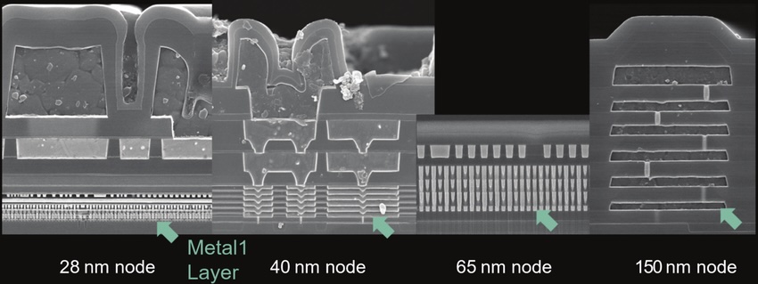
Moore's Law states that the number of transistors in CPUs will double every two years (sometimes incorrectly quoted as the speed doubling every two years).

The transistor density increase was initially supported by advances in the manufacturing processes, allowing for ever smaller transistor dimensions ("process node").

Table 1: Process node size shrinking over the years

Year	Product	Milestone	Process Node
1971	Intel 4004	First commercial microprocessor	10,000nm
1978	Intel 8086	Foundation of the x86 architecture	3,000nm
1989	Intel 486	First with on-chip floating point unit	1,000nm
1993	Intel Pentium	Superscalar architecture	800nm
2000	Intel Pentium 4	Peak of clock frequency scaling	180nm
2004		Dennard Scaling breaks down, clock speeds plateau	90nm
2006	Intel Core 2 Duo	Industry shifts to multicore	65nm
2012	Intel Ivy Bridge	First 3D FinFET transistors	22nm
2017	Apple A11	fFirst with dedicated neural engine	10nm
2019		TSMC volume production with EUV	7nm
2020	Apple M1	ARM displaces x86 in personal computing	5nm
2022		Intel cost per transistor increases for first time	4nm
2023	Apple M3	First consumer chip on 3nm node	3nm
2024		TSMC N2 gate-all-around transistors enter production	2nm

Moore's Law encountered fundamental material and manufacturing constraints as process nodes approached atomic scales:

90nm (2004)

Dennard Scaling held that shrinking transistors reduced voltage and current proportionally, keeping power density constant. At 90nm, the gate-oxide thickness was down to only a few atomic layers, and leakage current became significant as electrons tunnelled through the oxide via quantum effects. This is the era of "speed demons" like the Pentium 4 series, where clock frequencies plateaued at approximately 3–4 GHz before processors started to melt. The industry then transitioned to multicore architectures to sustain throughput through parallelism. A prime example of defeating frequency limits by exploiting parallelism was the Cell processor featured in the PlayStation 3, released in 2006.

7nm (2019)

As feature sizes pushed to 7nm and below, deep ultraviolet (DUV) immersion lithography could only keep up through increasingly complex multi-patterning, which drove up defect rates and cost. Extreme Ultraviolet (EUV) lithography — pioneered by ASML, the sole manufacturer of EUV scanners — was introduced for the most critical layers. TSMC was the first to deploy it in high-volume production, with its N7+ process in 2019. The added manufacturing complexity pushed cost per transistor up significantly.

3nm (2023)

Effective gate dielectrics thinned to just one to two atomic layers. At this scale, electron behaviour is dominated by quantum effects, including tunnelling through potential barriers, which compromises the deterministic switching behaviour that binary logic requires, turning manufacturing into a major challenge.

Process scaling alone could not sustain performance gains, so current innovation happens at the architecture level with the use of specialised accelerators (GPUs, TPUs, NPUs). That means gains became workload-specific, and require deliberate architectural choices.

Koomey's law states the number of computations per joule of energy dissipated doubles about every 2.6 years. Here's the numerical computing performance vs. power rating of the top 500 most energy efficient supercomputers over the last decade:

During the Dennard Scaling era, Koomey's Law and Moore's Law advanced together since denser transistors means higher efficiency. When Dennard Scaling broke down around 2004, the two diverged. Transistor counts continued rising but power density increased, temporarily slowing efficiency gains. Koomey's Law continued at a reduced rate, sustained by architectural and systems-level improvements rather than process scaling.

Nielsen's "Law of Internet Bandwidth" states that users' bandwidth grows by 50% per year.

Bandwidth grows more slowly than transistor density. This gap has structural consequences — computing capacity consistently outpaces the ability to move data, creating a persistent bottleneck between processing and communication. Applications must be designed around this asymmetry rather than assuming compute and bandwidth scale together.

As connections improved, content grew richer and applications more data-intensive, consuming available bandwidth and keeping perceived performance roughly constant. Web pages, video streaming and cloud applications expanded to fill whatever capacity was available.

Table 2: Time to download 10MB over the years

Technology	Year	Download speed	Seconds
Modem (V.34)	1994	28.8 kbit/s	2780
Modem (V.90)	1998	56.6 kbit/s	1410
ADSL (Consumer)	2000	256 kbit/s	313
ADSL (Consumer)	2000	512 kbit/s	156
ADSL (Consumer)	2000	1 Mbit/s	80
ADSL (Consumer)	2000	2 Mbit/s	40
ADSL (Max)	2006	8 Mbit/s	10
ADSL2+	2003	24 Mbit/s	3
3G (UMTS)	2001	384 kbit/s	208
3G (HSPA)	2006	7.2 Mbit/s	11
3G (HSPA+)	2008	21 Mbit/s	4
4G (LTE)	2009	150 Mbit/s	1
4G (LTE-A)	2011	300 Mbit/s	<0.5
5G (Sub-6GHz)	2018	400 Mbit/s	<0.5
5G (mmWave)	2019	2000 Mbit/s	<0.1

The transition from DSL to fibre and from 3G to 5G is sustaining the trend. Data-intensive applications such as video conferencing, cloud computing and large model inference kept demand ahead of supply, preserving the relevance of Nielsen's original observation. Still, bandwidth is a major constraint in distributed systems design and the economics of content delivery.

Latency, defined as the delay between transmiting a signal in one end and receiving on the other end, is bounded by two fundamental factors: the physical propagation of signals and the processing overhead at each stage.

Electrical signals in copper travel at roughly 60–70% of the speed of light, while optical signals in fiber travel at roughly 65% of the speed of light. At transatlantic scales, fiber link has a theoretical minimum of ~40ms imposed by the speed of light alone, before any processing occurs!

Within a processor, latency is determined by circuit depth and physical distance. Register access is measured in fractions of a nanosecond. Cache latency grows with distance from the core: L1 is on-die and fast, L3 is shared across cores and slower. RAM introduces additional delay from DRAM row activation and bus arbitration.

Moving onto storage, magnetic HDDs are dominated by seek time, where a physical read head has to move. SSDs eliminate mechanical movement but introduce controller processing and NAND flash charge sensing. NVMe reduces bus overhead by connecting directly to the CPU via PCIe.

Finally, on distant networks, each hop introduces propagation delay plus processing at routers, switches and protocol stacks. Wireless links add radio encoding and scheduling overhead. Satellite (GEO) latency is almost entirely propagation — signals must travel ~72,000km round trip to geostationary orbit.

We can see that latency spans ten orders of magnitude from CPU to satellite communication, so optimising a system can often begin by identifying which communication layer is a bottleneck.