Essential Color Science
(Draft)
"Color" may seem like a simple concept at first, but it's deceptive. Defining and interpreting color with precision involves a great deal of physics, mathematics, biology and even psychology. The science behind color impacts any industry that deals with light — photography, cinema, printing, eletrical engineering or medicine.
This article introduces color science from the ground up, condensing two centuries of discoveries into a coherent framework for how color has been perceived, specified, and reproduced. Little prior knowledge is assumed.
Light & Color
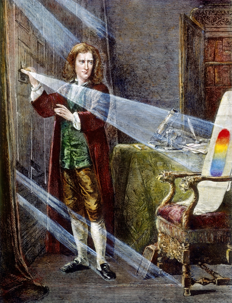
Sir Isaac Newton discovered that the sunlight could be split into its component colors when passed through a dispersive prism. The components can then be recombined using a second prism to produce white light. That means light is "additive" — in contrast to pigments that are "substractive", since combining different pigment colors makes black.
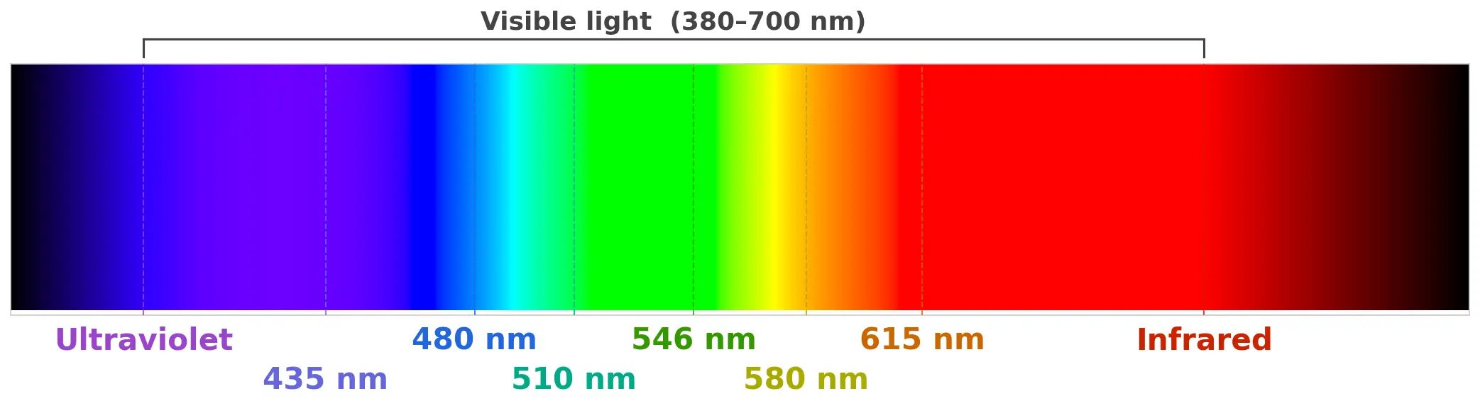
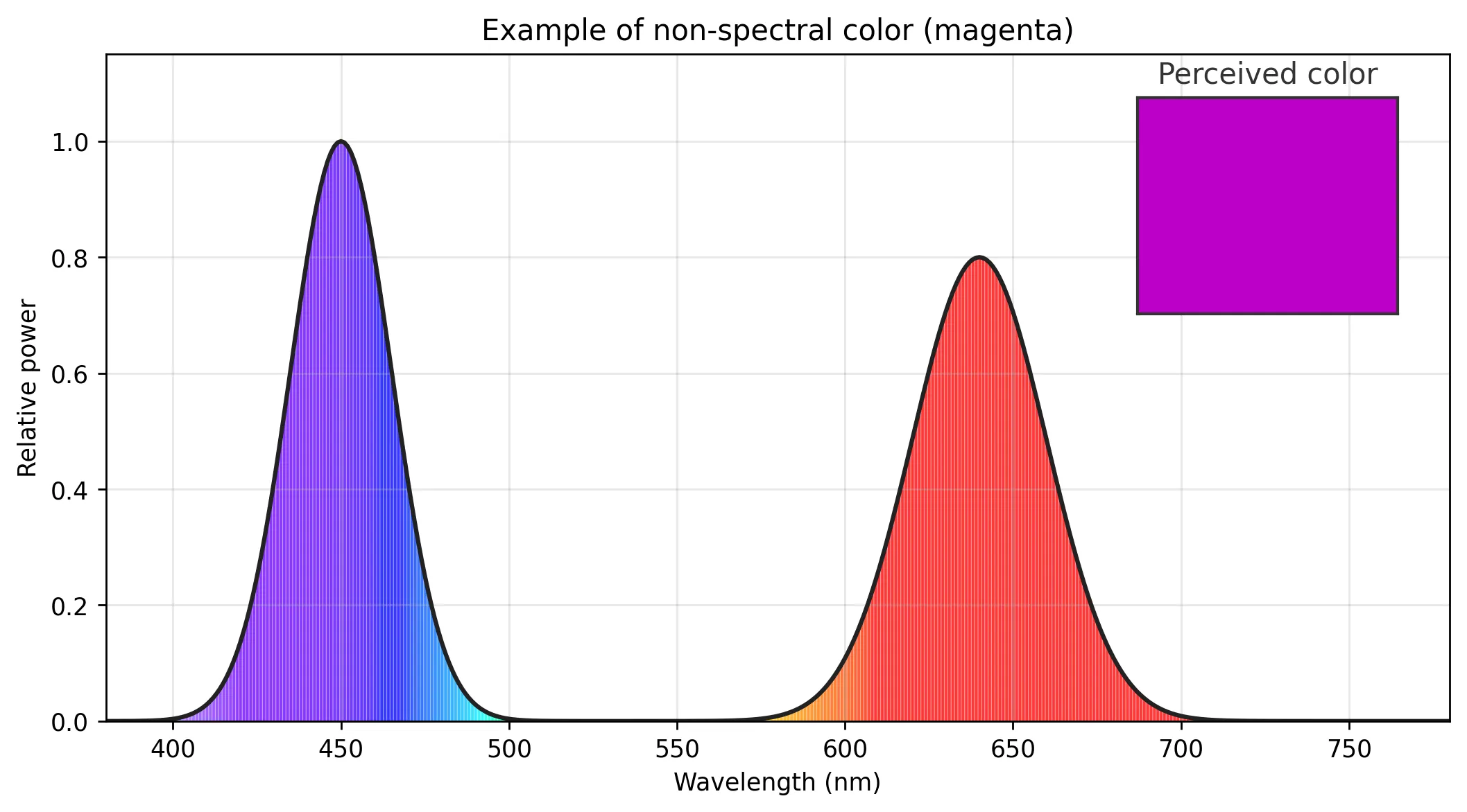
A spectral color is the color associated with a single wavelength of light. When viewed as a continuous spectrum, these colors are seen as the familiar rainbow. Conversely, a non-spectral color is the color made up by a combination of spectral colors.
Human Vision
Tristimulus values
The retina contains specialized cells known as rods and cells. Rods react mainly to light intensity, while cones react to certain wavelengths in different intensities.
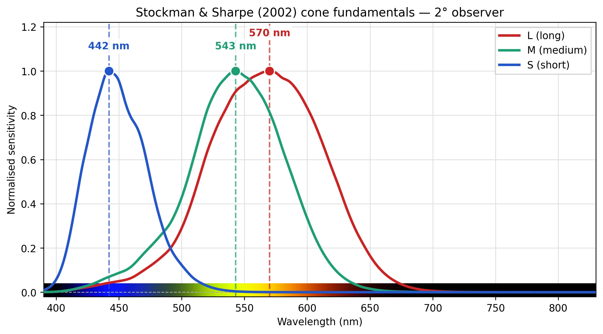
Humans with normal thrichromatic vision1 contain three types of cone cells, named long (L), medium (M) and short (S) after their peak response wavelengths. These responses don't correspond directly to colors as we normally understand, also depending on the encoding by the visual cortex and brain, and determined through experimentation. The discrete L,M,S responses to a certain light spectrum stimulus are known as tristimulus values.
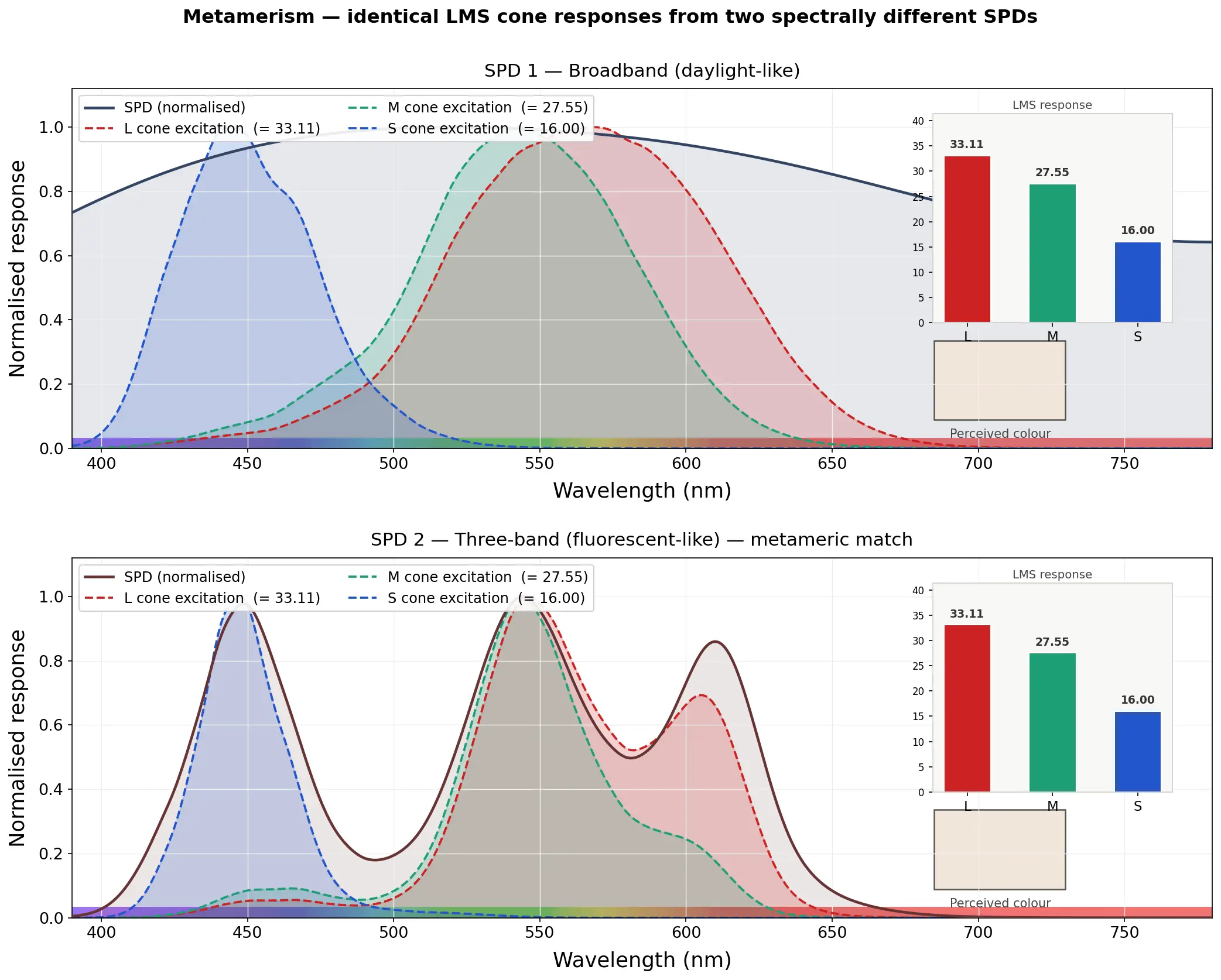
Metamerism
Given the light spectrum (an infinite-dimensional space) is projected to tristimulus values (3-dimensional), different light spectra may map to the same tristimulus. These indistinguishable light spectra are known as metamers.
Grassman laws
Hermann Graßmann (Grassmann) presented in "On the Theory of Color Mixing" (1853)2 an algebra to describe light mixing, obeying the following laws:
- Additivity
- Given lights \(\{a, b, z\}\), if \(a = b\) (metamers), then \(a + z = b + z\) (also metamers).
- Proportionality
- Given lights \(\{a, b\}\) and a constant \(m\), if \(a = b\) (metamers), then \(a * m = b * m\) (also metamers).
- Transitivity
- Given lights \(\{a,b,c\}\), if \(a = b\) and \(b = c\), then \(a = b = c\) (all colors are metameric).
Future color experiments were based on this theory, performed by Hermann von Helmholtz and James Clerk Maxwell in the 1850's, and the experiments by Wright (1928) and Guild (1931).
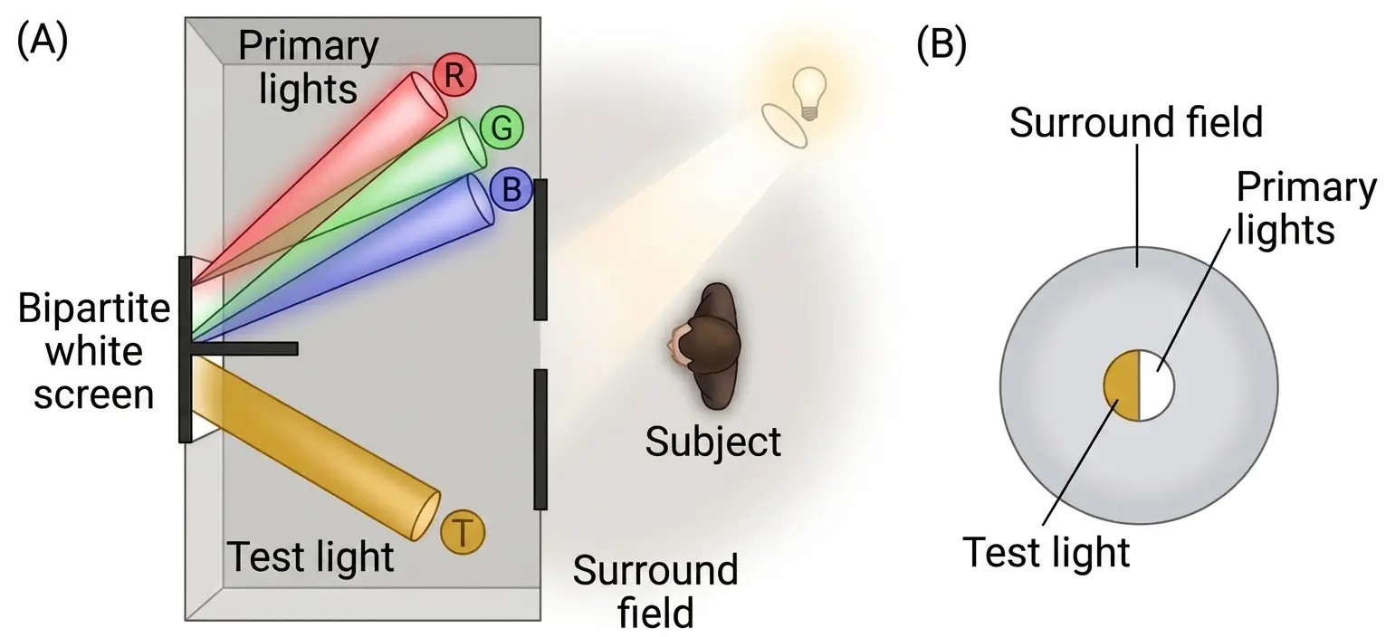
Color matching experiments
In these experiments, an observer sees a bipartite white screen through an aperture, onto which the light of different lamps will be projected. At one side, a target light \(T\) generates a certain color impression in the observer, while another side is illuminated by three monochromatic lights \(R, G, B\) that mixed together generate the color impression \(C\). The objective is to match the color impresions from both sides by adjusting the power of the three monochromatic lights, or in some cases, mixing one of the monochromatic lights with the target.
Luminance perception
The human visual system responds to luminance approximately logarithmically. The Weber-Fechner law states that the perceived change in a stimulus is proportional to the ratio of the change to the initial intensity, not to the absolute difference. That is the same as stating that stimulus increases have to follow a geometric progression for the perception to follow an arithmetic progression.
Photographic film exhibits a strikingly similar response. The Hurter-Driffield (1890) curve modeled how the optical density of a developed emulsion is approximately proportional to the logarithm of the exposure (the product of luminance and time). The curve has three regions: a toe where the emulsion barely responds to low exposures, a straight-line section where density rises proportionally with log exposure, and a shoulder where the emulsion saturates and additional light produces diminishing returns. In the straight-line portion, the film acts as a logarithmic encoder of scene luminance.
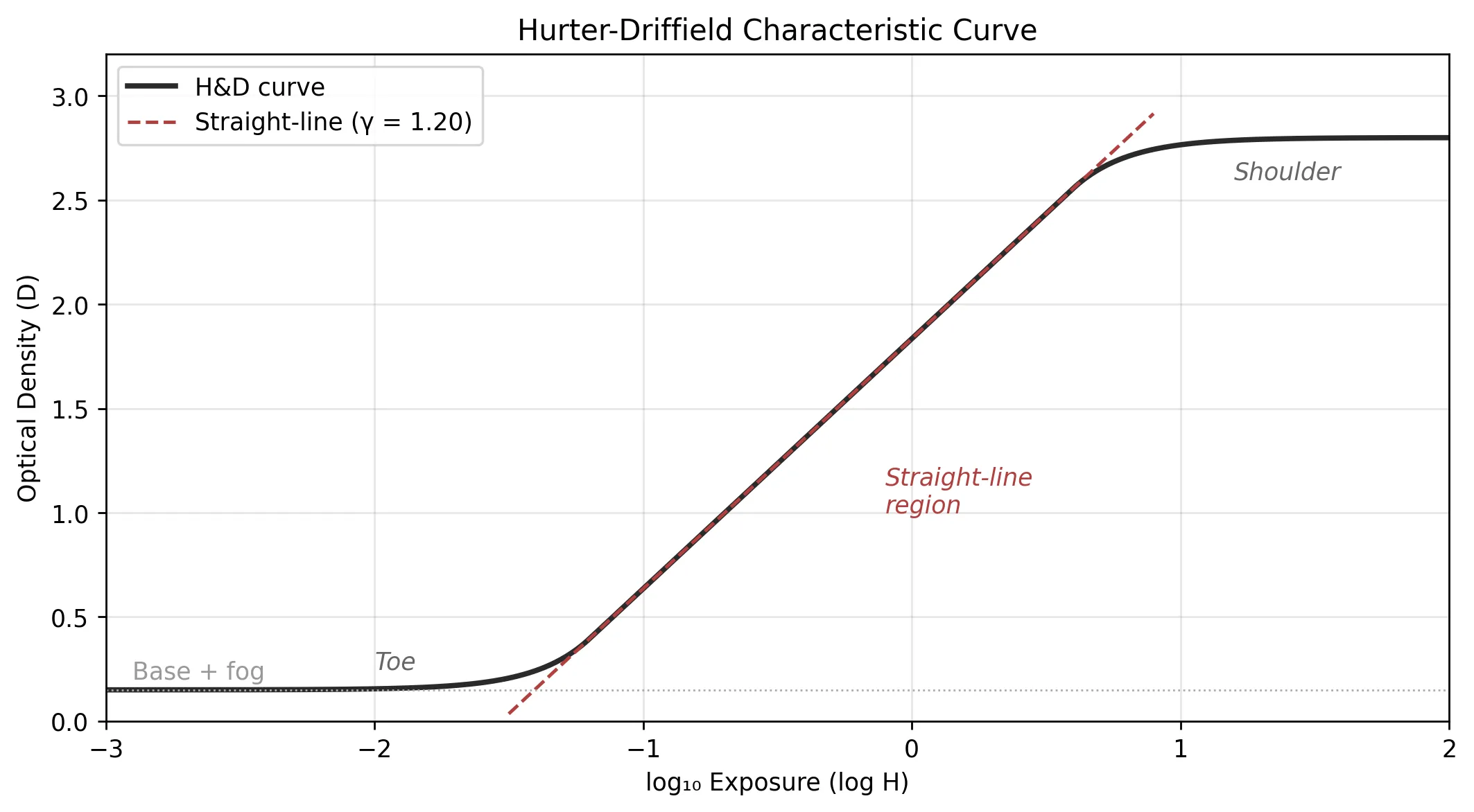
The slope of the straight-line segment is known as the film's gamma. A gamma greater than 1 increases contrast; less than 1 compresses it. Different film stocks and development processes yield different gamma values. A high-contrast copy film might have a gamma of 2.0 or more, while a negative film intended for pictorial work might sit around 0.6, relying on the print stage to restore contrast.
CIE 1931
In 1931, the International Commission on Illumination (CIE) published the CIE 1931 color which define the relationship between the visible spectrum and human color vision3. The CIE color spaces are mathematical models that comprise a "standard observer", which is a static idealization of the color vision of a normal human.
The CIE color spaces were created using data from a series of experiments by William David Wright and John Guild. The experimental results were combined, creating the CIE RGB color space.
CIE RGB
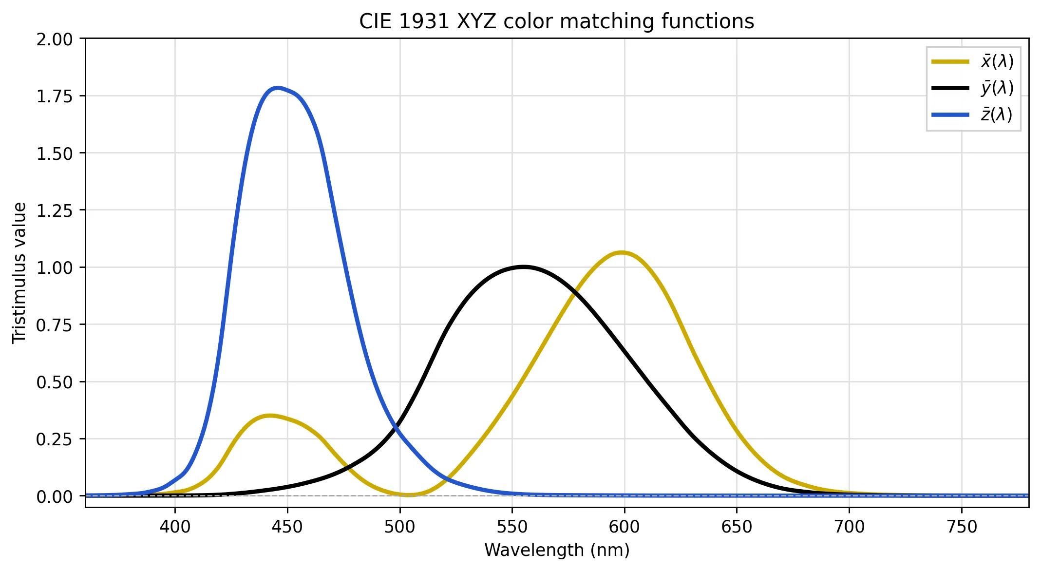
The CIE RGB is the colorspace based on the standardized color matching functions \(\bar{r}(\lambda), \bar{g}(\lambda), \bar{b}(\lambda)\) obtained using three monochromatic light sources (primaries) at standardized wavelengths of 700 nm (red), 546.1 nm (green) and 435.8 nm (blue) 4.
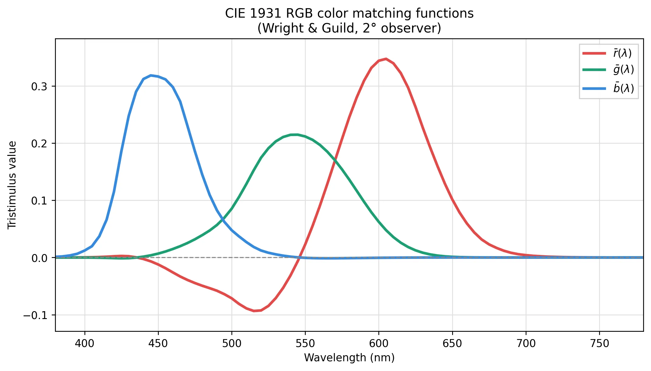
The distribution of spectral energy is normalized and adding all color matching functions equals 1. Negative values in the graph indicate primary colors have to be mixed with the target color before color matching.
CIE rg
The CIE rg is a two-dimensional space derived from RGB that determines the chromaticity coordinates in a plane and discards the luminance. A color is represented by the proportion of red, green, and blue in the color, rather than by the intensity of each.
\begin{aligned} r={\frac {R}{R+G+B}}\\ g={\frac {G}{R+G+B}}\\ b={\frac {B}{R+G+B}}\\ r+g+b=1 \end{aligned}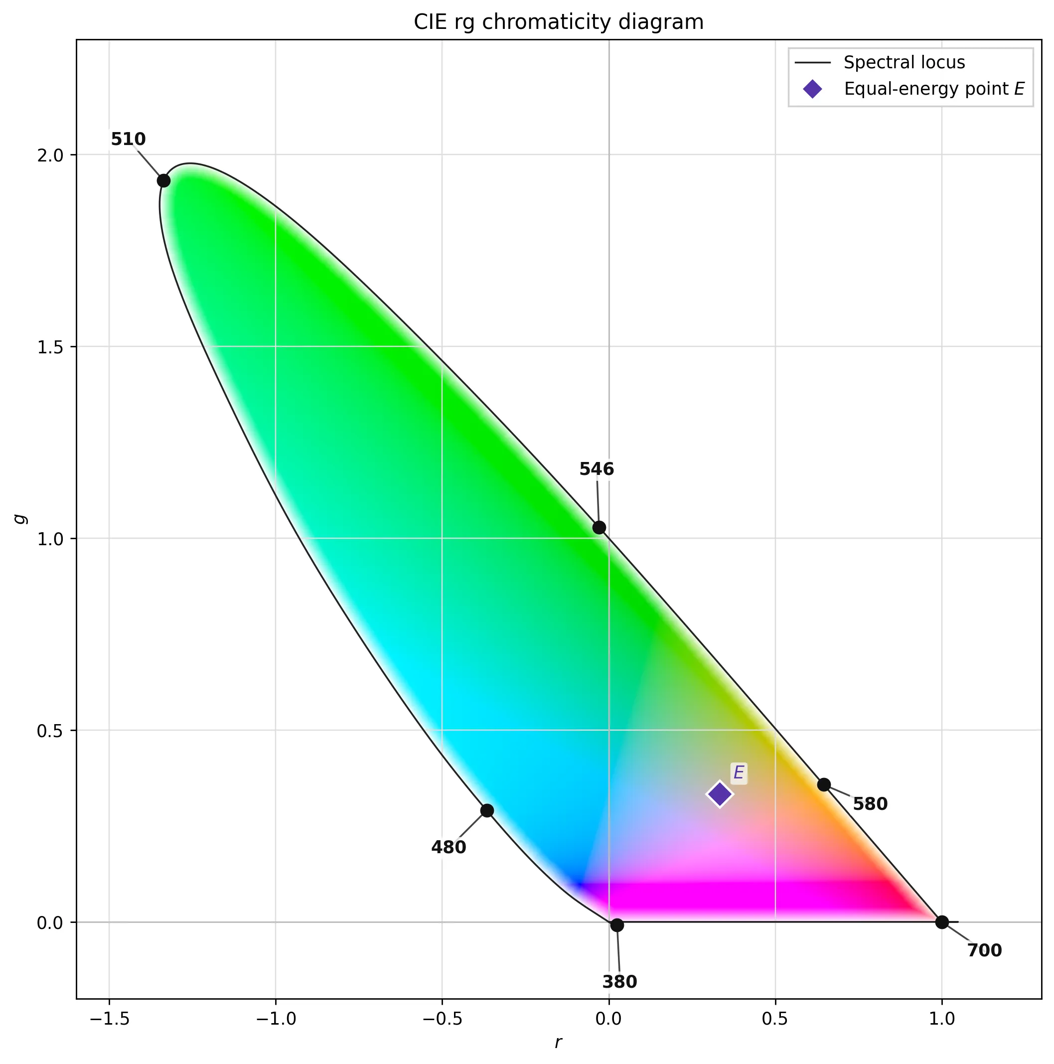
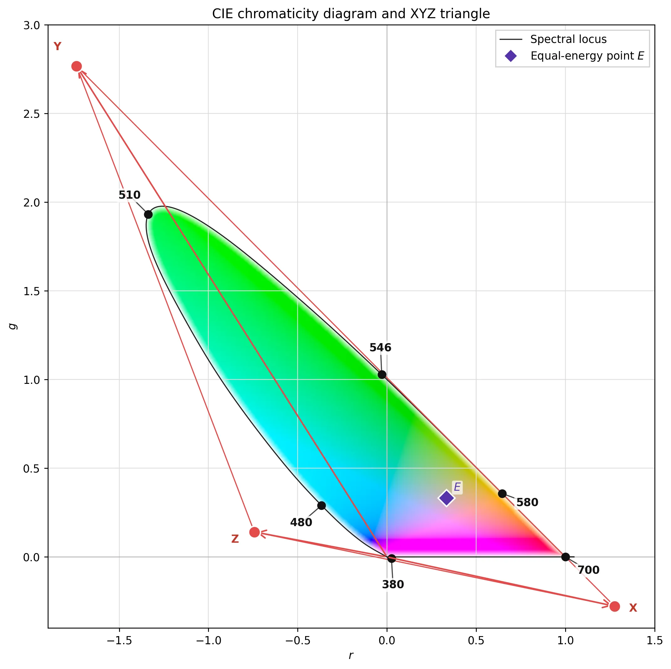
CIE XYZ
The CIE XYZ tristimulus values are a device-invariant representation of color 5. It serves as a standard reference against which many other color spaces are defined.
It is defined as a conveninent linear transformation of the CIE 1931 RGB colorspace, such that:
- \(\bar{x}(\lambda), \bar{y}(\lambda), \bar{z}(\lambda) \in \mathbb {R} _{>0}\)
- \(\{(x, y) \in \mathbb{R}^2 \mid x \geq 0,\ y \geq 0,\ x + y \leq 1\}\); so the gamut of colors will lie inside a unit triangle
- \(\bar{x}(E) = \bar{y}(E) = \bar{z}(E) = 1/3\); where \(E\) is the equal-energy white point
In the CIE 1931 model, Y is the luminance, Z is quasi-equal to blue (of CIE RGB), and X is a mix of the three CIE RGB curves chosen to be nonnegative. Setting Y as luminance has the useful result that for any given Y value, the XZ plane will contain all possible chromaticities at that luminance.
The color matching functions \(\bar{r}(\lambda), \bar{g}(\lambda), \bar{b}(\lambda)\) are negative at certain wavelengths to allow for any monochromatic sample to be matched. This is why in the rg chromaticity diagram the spectral locus extents into the negative r direction and ever so slightly into the negative g direction. Avoiding negative color coordinate values prompted the change from to rg to xy.
CIE xyY
Three dimensional color can be divided into two parts: brightness and chromaticity. For example, the color white is a bright color, while the color grey is considered to be a less bright version of that same white. In other words, the chromaticity of white and grey are the same while their brightness differs. The CIE xyY color space was deliberately designed so that the Y parameter is also a measure of the luminance of a color. The chromaticity is then specified by the two derived parameters x and y, two of the three normalized values derived from the tristimulus values X, Y, and Z.
\begin{aligned} x&={\frac {X}{X+Y+Z}}\\ y&={\frac {Y}{X+Y+Z}}\\ z&={\frac {Z}{X+Y+Z}}=1-x-y \end{aligned}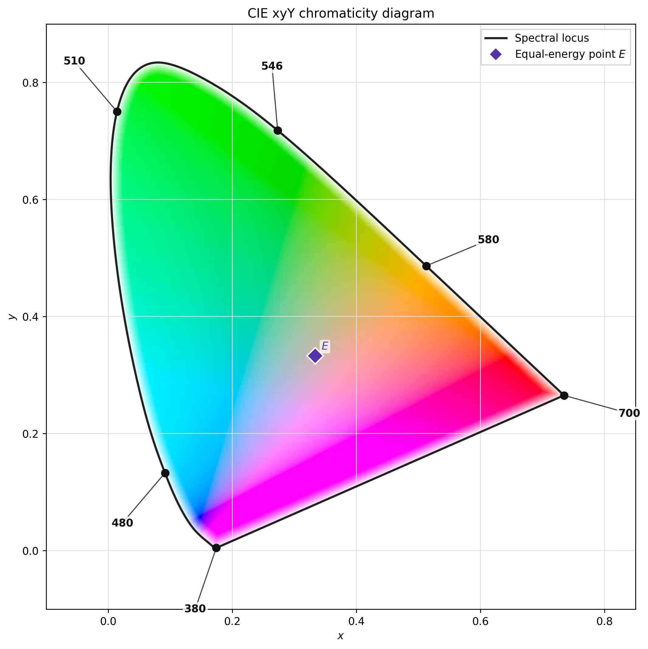
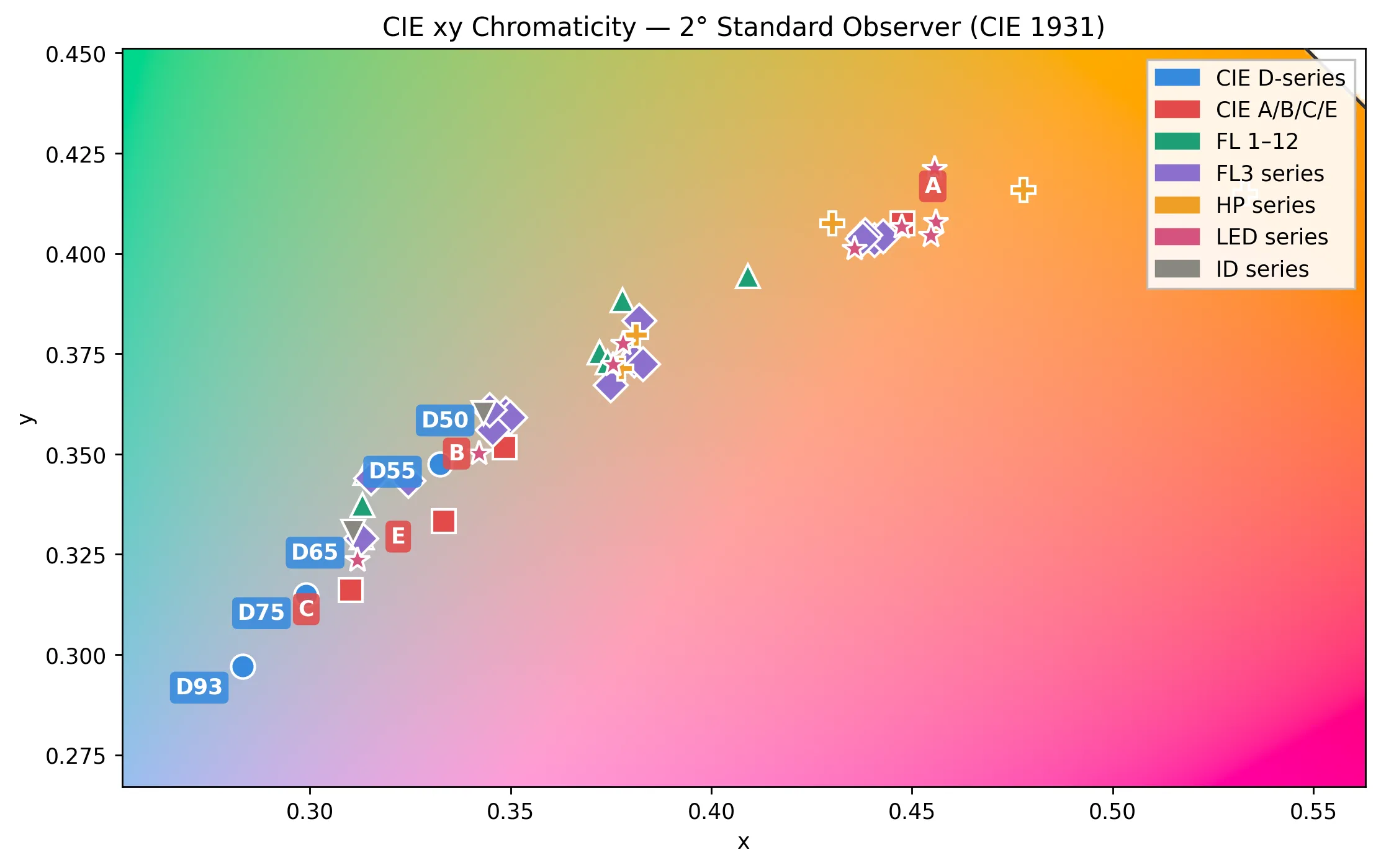
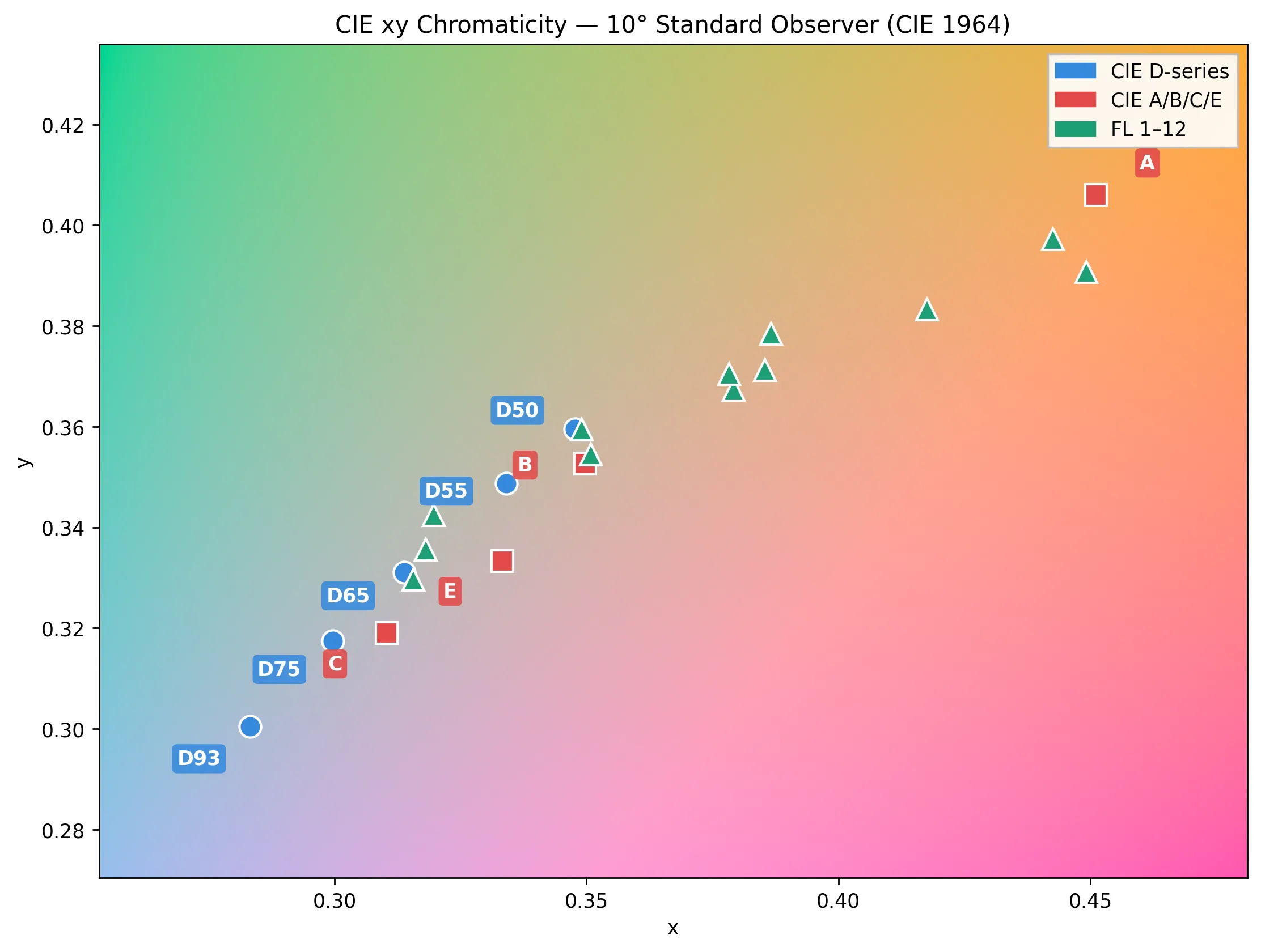
CIE Illuminants
When Y = 1 is defined as the brightest white, the corresponding chromaticity values for x and y can then be inferred using the standard illuminants.
Illuminants A, B, and C were standardized in 1931, with the intention of respectively representing average incandescent light, direct sunlight, and average daylight. Illuminants D (1967) represent variations of daylight, illuminant E is the equal-energy illuminant, while illuminants F (2004) represent fluorescent lamps of various composition.
| Illuminant | x 2° | y 2° | x 10° | y 10° | CCT6 (K) | Note |
|---|---|---|---|---|---|---|
| A | 0.44758 | 0.40745 | 0.45117 | 0.40594 | 2856 | incandescent / tungsten |
| B | 0.34842 | 0.35161 | 0.34980 | 0.35270 | 4874 | obsolete, direct sunlight at noon |
| C | 0.31006 | 0.31616 | 0.31039 | 0.31905 | 6774 | obsolete, average / North sky daylight NTSC 1953, PAL-M |
| D50 | 0.34567 | 0.35850 | 0.34773 | 0.35952 | 5003 | horizon light, ICC profile PCS |
| D55 | 0.33242 | 0.34743 | 0.33411 | 0.34877 | 5503 | mid-morning / mid-afternoon daylight |
| D65 | 0.31272 | 0.32903 | 0.31382 | 0.33100 | 6504 | noon daylight: television, sRGB color space |
| D75 | 0.29902 | 0.31485 | 0.29968 | 0.31740 | 7504 | North sky daylight |
| D93 | 0.28315 | 0.29711 | 0.28327 | 0.30043 | 9305 | high-efficiency blue phosphor monitors, BT.2035, NTSC-J |
| E | 0.33333 | 0.33333 | 0.33333 | 0.33333 | 5454 | equal energy |
| FL1 | 0.31310 | 0.33727 | 0.31811 | 0.33559 | 6430 | daylight fluorescent |
| FL2 | 0.37208 | 0.37529 | 0.37925 | 0.36733 | 4230 | cool white fluorescent |
| FL3 | 0.40910 | 0.39430 | 0.41761 | 0.38324 | 3450 | white fluorescent |
| FL4 | 0.44018 | 0.40329 | 0.44920 | 0.39074 | 2940 | warm white fluorescent |
| FL5 | 0.31379 | 0.34531 | 0.31975 | 0.34246 | 6350 | daylight fluorescent |
| FL6 | 0.37790 | 0.38835 | 0.38660 | 0.37847 | 4150 | light white fluorescent |
| FL7 | 0.31292 | 0.32933 | 0.31569 | 0.32960 | 6500 | D65 simulator, daylight simulator |
| FL8 | 0.34588 | 0.35875 | 0.34902 | 0.35939 | 5000 | D50 simulator, Sylvania F40 Design 50 |
| FL9 | 0.37417 | 0.37281 | 0.37829 | 0.37045 | 4150 | cool white deluxe fluorescent |
| FL10 | 0.34609 | 0.35986 | 0.35090 | 0.35444 | 5000 | Philips TL85, Ultralume 50 |
| FL11 | 0.38052 | 0.37713 | 0.38541 | 0.37123 | 4000 | Philips TL84, Ultralume 40 |
| FL12 | 0.43695 | 0.40441 | 0.44256 | 0.39717 | 3000 | Philips TL83, Ultralume 30 |
| FL3.1 | 0.4407 | 0.4033 | 2932 | standard halophosphate | ||
| FL3.2 | 0.3808 | 0.3734 | 3965 | standard halophosphate | ||
| FL3.3 | 0.3153 | 0.3439 | 6280 | standard halophosphate | ||
| FL3.4 | 0.4429 | 0.4043 | 2904 | DeLuxe type | ||
| FL3.5 | 0.3749 | 0.3672 | 4086 | DeLuxe type | ||
| FL3.6 | 0.3488 | 0.3600 | 4894 | DeLuxe type | ||
| FL3.7 | 0.4384 | 0.4045 | 2979 | Three-band | ||
| FL3.8 | 0.3820 | 0.3832 | 4006 | Three-band | ||
| FL3.9 | 0.3499 | 0.3591 | 4853 | Three-band | ||
| FL3.10 | 0.3455 | 0.3560 | 5000 | Three-band | ||
| FL3.11 | 0.3245 | 0.3434 | 5854 | Three-band | ||
| FL3.12 | 0.4377 | 0.4037 | 2984 | Multi-band | ||
| FL3.13 | 0.3830 | 0.3724 | 3896 | Multi-band | ||
| FL3.14 | 0.3447 | 0.3609 | 5045 | Multi-band | ||
| FL3.15 | 0.3127 | 0.3290 | 6509 | D65 Simulator | ||
| HP1 | 0.533 | 0.415 | 1959 | Standard high pressure sodium lamp | ||
| HP2 | 0.4778 | 0.4158 | 2506 | Color-enhanced high-pressure sodium lamp | ||
| HP3 | 0.4302 | 0.4075 | 3144 | High pressure metal halide lamp | ||
| HP4 | 0.3812 | 0.3797 | 4002 | High pressure metal halide lamp | ||
| HP5 | 0.3776 | 0.3713 | 4039 | High pressure metal halide lamp | ||
| LED-B1 | 0.4560 | 0.4078 | 2733 | phosphor-converted blue | ||
| LED-B2 | 0.4357 | 0.4012 | 2998 | phosphor-converted blue | ||
| LED-B3 | 0.3756 | 0.3723 | 4103 | phosphor-converted blue | ||
| LED-B4 | 0.3422 | 0.3502 | 5109 | phosphor-converted blue | ||
| LED-B5 | 0.3118 | 0.3236 | 6598 | phosphor-converted blue | ||
| LED-BH1 | 0.4474 | 0.4066 | 2851 | mixing of phosphor-converted blue LED and red LED (blue-hybrid) | ||
| LED-RGB1 | 0.4557 | 0.4211 | 2840 | mixing of red, green, and blue LEDs | ||
| LED-V1 | 0.4548 | 0.4044 | 2724 | phosphor-converted violet | ||
| LED-V2 | 0.3781 | 0.3775 | 4070 | phosphor-converted violet | ||
| ID50 | 0.3432 | 0.3602 | 5098 | natural indoor daylight | ||
| ID65 | 0.3107 | 0.3307 | 6603 | natural indoor daylight |
Device-dependent definitions
Transfer functions
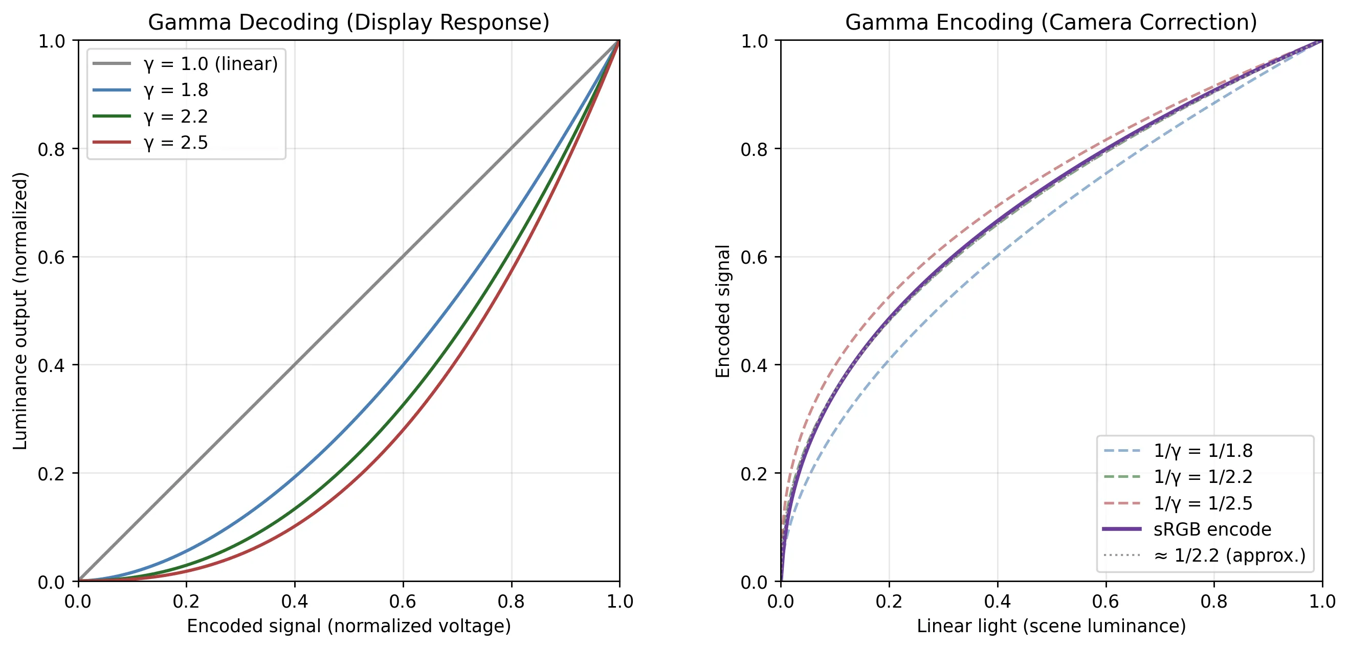
Gamma
When the cathode ray tube power-law response was characterized, the exponent was called gamma by direct analogy with the gamma parameter from photography. A gamma-encoded signal dedicates more code values to the dark regions where the eye discriminates finely, and fewer to the bright regions where it does not, achieving an efficient perceptual encoding without requiring more bits or bandwidth.
Linear
The simplest possible transfer function, a linear encoding stores values directly proportional to the the scene luminance. This is the primary encoding for RAW formats used by photographic cameras, and is a direct consequence of the linear response from CMOS sensors.
Linear encoding is also the natural choice for physically-based rendering, compositing, and any operation that involves adding or multiplying light values in computer graphics.
Since linear encoding does not consider luminance perception, it is inneficient in terms of space. Given a 14-stop scene quantized in 14 bits, the brightest stop occupies the range \([8192, 16383]\), which is half of all the available range. The next stop occupies \([4096, 8191]\), and so on. By the time we reach the darkest stop, only 1 code value remains. So this encoding scheme alllocates more data space to highlights (where perceptual sensitivity is lower) and less data space to shadows (where perceptual sensitivity is higher).
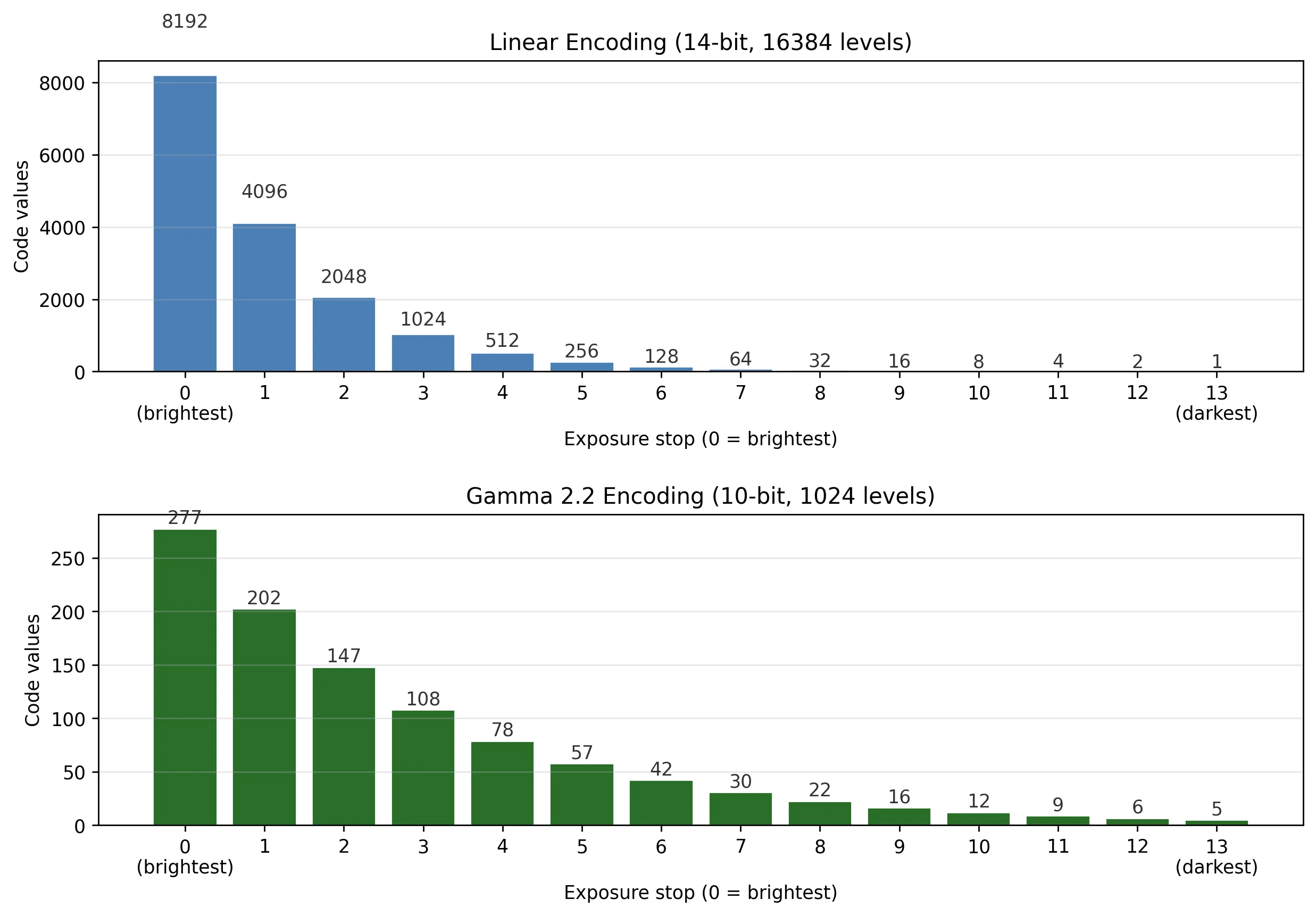
8192 values to the brightest stop and only 1 to the darkest, while gamma redistributes code values more evenly.This is why RAW files demand higher bit depths than display-referred formats. A 14-bit linear file and a 10-bit gamma-encoded file contain a comparable number of perceptually distinguishable steps in the shadows, despite the linear file being four times larger. The 4096 extra levels bought by those additional bits are almost entirely consumed by the highlights, where they contribute little visible benefit.
Logarithmic
When Kodak designed the Cineon file format in the early 1990s for scanning film negatives, they adopted a 10-bit logarithmic encoding (the "printing density" scale) that better preserved the film's logarithmic response. This digital pipeline (scan to Cineon, grade, film-out) produced good results because the encoding matched the medium.
With the advent of digital cameras, manufacturers wanted an equivalent transfer function to avoid the quantization issues of a simple linear encoding. This ideal encoding should map the sensor's linear output into a logarithmic code-value space, capturing the full dynamic range of the sensor.
| Year | Vendor | Encoding | Bit depth |
|---|---|---|---|
| 2004 | Sony | S-Log | 10 |
| 2010 | ARRI | LogC | 10 |
| 2011 | Sony | S-Log2 | 10 |
| 2011 | Canon | C-Log | 10 |
| 2013 | Sony | S-Log3 | 10 |
| 2017 | RED | Log3G10 | 10 or 16 |
E.g., S-Log3, the current standard in Sony's cinema cameras, is defined piecewise:
\begin{aligned} V = \begin{cases} \dfrac{171.2102946929 - 95.0}{0.01125} \cdot x + 95.0 & x < 0.01125 \\[6pt] 420.0 + \log_{10}\!\left(\dfrac{x + 0.01}{0.18 + 0.01}\right) \cdot 261.5 & x \geq 0.01125 \end{cases} \end{aligned}where \(x\) is the linear scene value (with 0.18 corresponding to middle grey) and \(V\) is the 10-bit code value. The linear segment near black prevents the logarithm from diverging, serving the same purpose as the linear toe in sRGB — though at a very different scale.
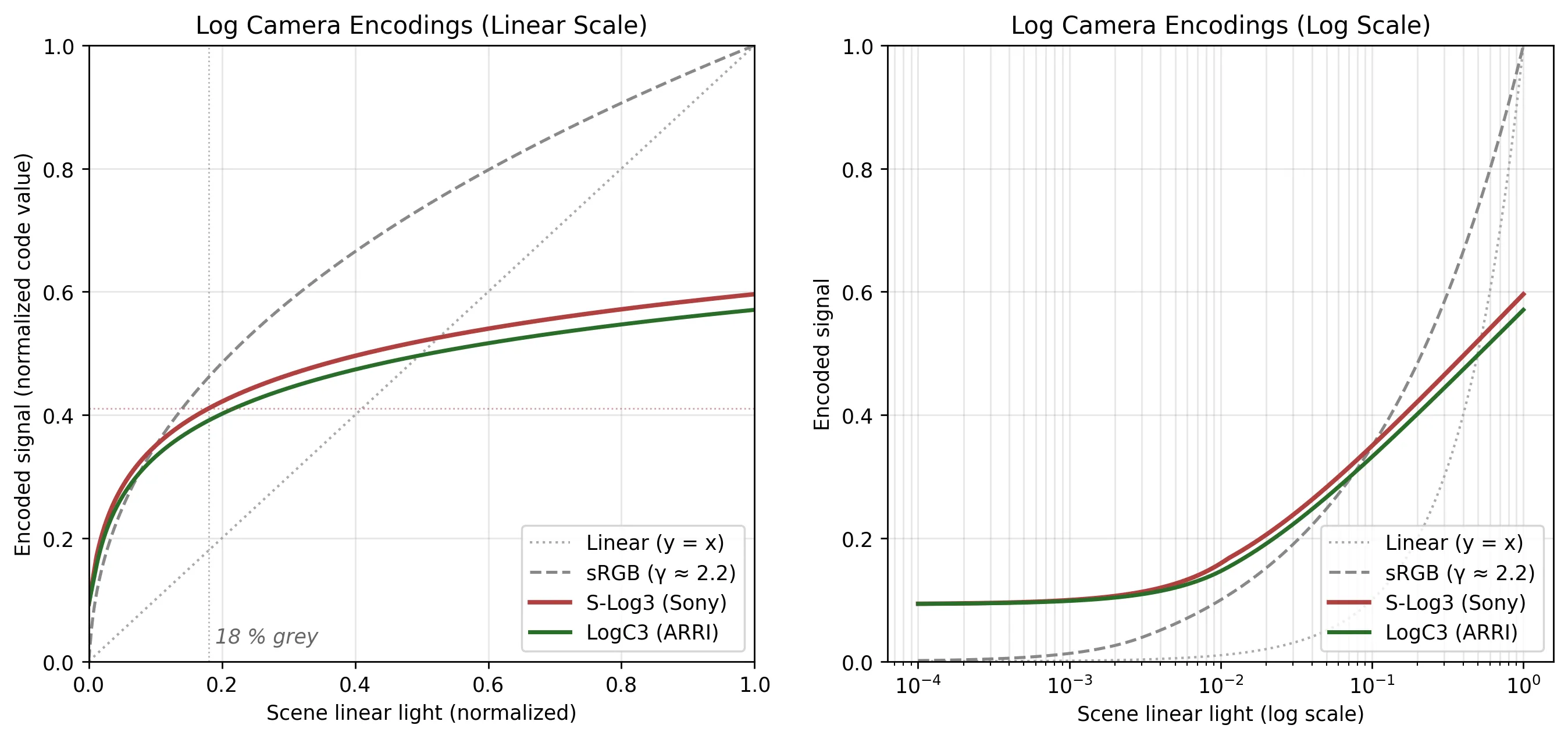
The footage recorded in logarithmic encoding is not intended for direct viewing, since it would appear flat in contrast. The log encoding is a scene-referred capture format, preserving the full dynamic range of the sensor so that a colorist can map it to any output medium in post-production.
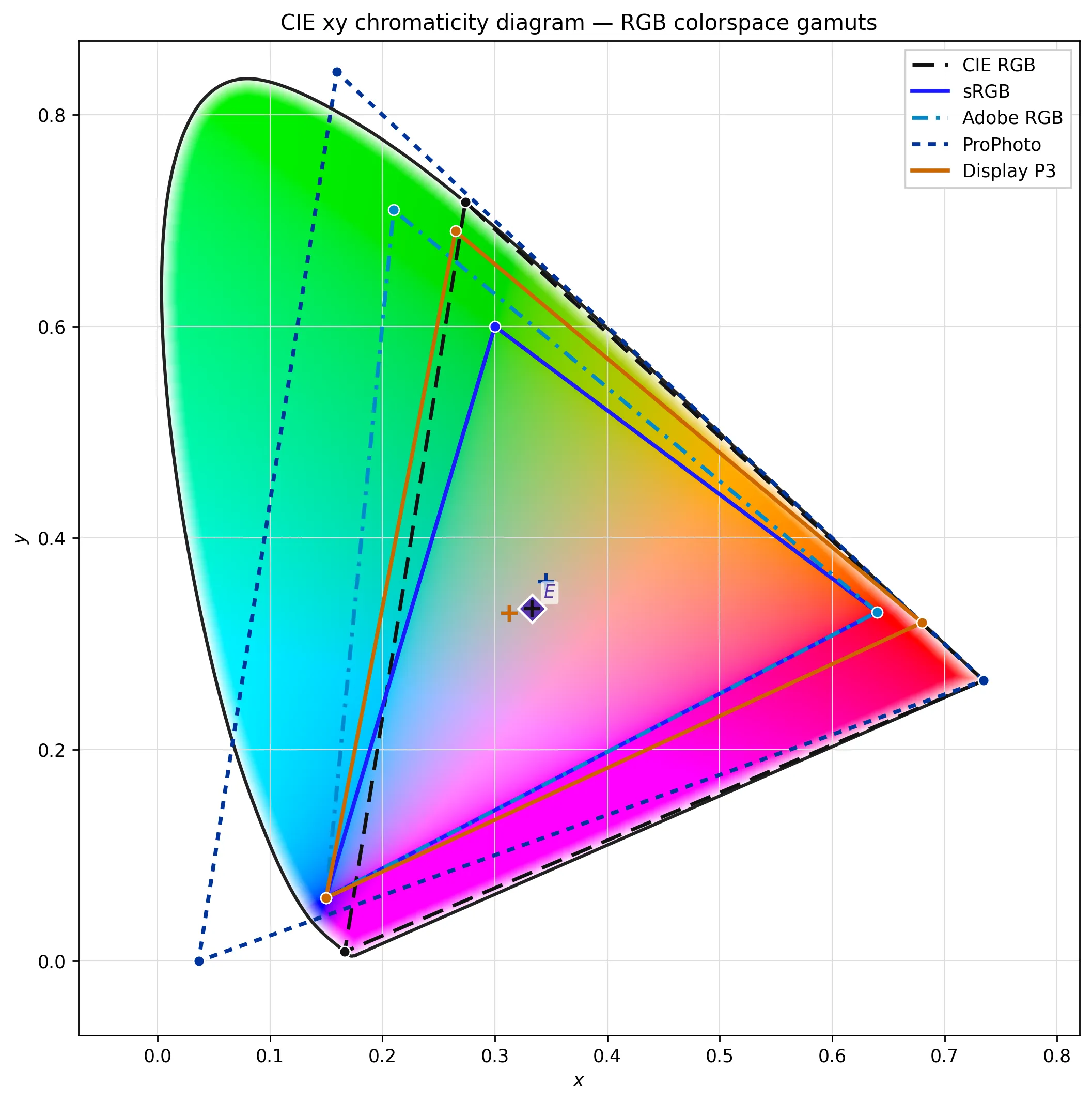
RGB working spaces
By choosing different RGB primaries (basis vectors in 3-dimensional space) and white-point other than CIE 1931 RGB's, new volumes can be defined spanning a different gamut8 of colors. This allows trading-off color reproduction accuracy and data encoding sizes, depending on the intended application.
When a RGB colorspace specifies a display device or media , it's also known as output space. When a RGB colorspace is used as an intermediate step in a image manipulation pipeline, it can also be named working space. Some examples are standard RGB (sRGB)
Early examples of RGB color spaces came with the adoption of the NTSC color television standard in 1953 across North America, followed by PAL and SECAM covering the rest of the world. These early RGB spaces were defined in part by the phosphor used by CRTs in use at the time, and the gamma of the electron beam. While these color spaces reproduced the intended colors using additive red, green, and blue primaries, the broadcast signal itself was encoded from RGB components to a composite signal such as YIQ, and decoded back by the receiver into RGB signals for display.
HDTV uses the BT.709 color space, later repurposed for computer monitors as sRGB. Both use the same color primaries and white point, but different transfer functions. The gamut of these spaces is limited, covering only 35.9% of the CIE 1931 gamut 9. While this allows the use of a limited bit depth without causing color banding, and therefore reduces transmission bandwidth, it also prevents the encoding of deeply saturated colors that might be available in an alternate color spaces. Adobe RGB and ProPhoto, which are intended as working spaces, are designed with expanded gamuts to address this issue, however this does not mean the larger space has 'more colors". The numerical quantity of colors is related to data encoding bit depth and not the size or shape of the gamut. There's a fundamental precision trade-off between a wide gamut space encoded as low bit depth. More recent color spaces such as Rec. 2020 for UHD-TVs define an extremely large gamut covering 63.3% of the CIE 1931 space 10. This standard was forward-compatible, since it wasn't realizable with LCD panel technology at the time.
| Colorspace | Gamma | Illuminant | Red xy | Green xy | Blue xy |
|---|---|---|---|---|---|
| Adobe RGB (1998) | 2.2 | D65 | 0.6400 0.3300 | 0.2100 0.7100 | 0.1500 0.0600 |
| Apple RGB | 1.8 | D65 | 0.6250 0.3400 | 0.2800 0.5950 | 0.1550 0.0700 |
| CIE XYZ | ~ | E | 1.0000 0.0000 | 0.0000 1.0000 | 0.0000 0.0000 |
| CIE RGB | ~ | E | 0.7350 0.2650 | 0.2740 0.7170 | 0.1670 0.0090 |
| Display P3 | ≈2.211 | D65 | 0.6800 0.3200 | 0.2650 0.6900 | 0.1500 0.0060 |
| NTSC RGB | 2.2 | C | 0.6700 0.3300 | 0.2100 0.7100 | 0.1400 0.0800 |
| PAL/SECAM RGB | 2.2 | D65 | 0.6400 0.3300 | 0.2900 0.6000 | 0.1500 0.0600 |
| ProPhoto RGB | 1.8 | D50 | 0.7347 0.2653 | 0.1596 0.8404 | 0.0366 0.0001 |
| sRGB | ≈2.211 | D65 | 0.6400 0.3300 | 0.3000 0.6000 | 0.1500 0.0600 |
| Wide Gamut RGB | 2.2 | D50 | 0.7350 0.2650 | 0.1150 0.8260 | 0.1570 0.0180 |
| Colorspace | Illuminant | RGB to XYZ [M] | XYZ to RGB [M]⁻¹ | ||||
|---|---|---|---|---|---|---|---|
| Adobe RGB (1998) | D65 | 0.5767309 | 0.1855540 | 0.1881852 | 2.0413690 | −0.5649464 | −0.3446944 |
| 0.2973769 | 0.6273491 | 0.0752741 | −0.9692660 | 1.8760108 | 0.0415560 | ||
| 0.0270343 | 0.0706872 | 0.9911085 | 0.0134474 | −0.1183897 | 1.0154096 | ||
| Apple RGB | D65 | 0.4497288 | 0.3162486 | 0.1844926 | 2.9515373 | −1.2894116 | −0.4738445 |
| 0.2446525 | 0.6720283 | 0.0833192 | −1.0851093 | 1.9908566 | 0.0372026 | ||
| 0.0251848 | 0.1411824 | 0.9224628 | 0.0854934 | −0.2694964 | 1.0912975 | ||
| CIE RGB | E | 0.4887180 | 0.3106803 | 0.2006017 | 2.3706743 | −0.9000405 | −0.4706338 |
| 0.1762044 | 0.8129847 | 0.0108109 | −0.5138850 | 1.4253036 | 0.0885814 | ||
| 0.0000000 | 0.0102048 | 0.9897952 | 0.0052982 | −0.0146949 | 1.0093968 | ||
| Display P3 | D65 | 0.4865709 | 0.2656677 | 0.1982173 | 2.4934969 | −0.9313836 | −0.4027108 |
| 0.2289746 | 0.6917385 | 0.0792869 | −0.8294890 | 1.7626641 | 0.0236247 | ||
| 0.0000000 | 0.0451134 | 1.0439444 | 0.0358458 | −0.0761724 | 0.9568845 | ||
| NTSC RGB | C | 0.6068909 | 0.1735011 | 0.2003480 | 1.9099961 | −0.5324542 | −0.2882091 |
| 0.2989164 | 0.5865990 | 0.1144845 | −0.9846663 | 1.9991710 | −0.0283082 | ||
| 0.0000000 | 0.0660957 | 1.1162243 | 0.0583056 | −0.1183781 | 0.8975535 | ||
| PAL/SECAM RGB | D65 | 0.4306190 | 0.3415419 | 0.1783091 | 3.0628971 | −1.3931791 | −0.4757517 |
| 0.2220379 | 0.7066384 | 0.0713236 | −0.9692660 | 1.8760108 | 0.0415560 | ||
| 0.0201853 | 0.1295504 | 0.9390944 | 0.0678775 | −0.2288548 | 1.0693490 | ||
| ProPhoto RGB | D50 | 0.7976749 | 0.1351917 | 0.0313534 | 1.3459433 | −0.2556075 | −0.0511118 |
| 0.2880402 | 0.7118741 | 0.0000857 | −0.5445989 | 1.5081673 | 0.0205351 | ||
| 0.0000000 | 0.0000000 | 0.8252100 | 0.0000000 | 0.0000000 | 1.2118128 | ||
| sRGB | D65 | 0.4124564 | 0.3575761 | 0.1804375 | 3.2404542 | −1.5371385 | −0.4985314 |
| 0.2126729 | 0.7151522 | 0.0721750 | −0.9692660 | 1.8760108 | 0.0415560 | ||
| 0.0193339 | 0.1191920 | 0.9503041 | 0.0556434 | −0.2040259 | 1.0572252 | ||
| Wide Gamut RGB | D50 | 0.7161046 | 0.1009296 | 0.1471858 | 1.4628067 | −0.1840623 | −0.2743606 |
| 0.2581874 | 0.7249378 | 0.0168748 | −0.5217933 | 1.4472381 | 0.0677227 | ||
| 0.0000000 | 0.0517813 | 0.7734287 | 0.0349342 | −0.0968930 | 1.2884099 |
Chromatic Adaptation
Chromatic adaptation is the human visual system's ability to adjust to changes in illumination in order to preserve the appearance of object colors. It is responsible for the stable appearance of object colors despite the wide variation of light which might be reflected from an object and observed by our eyes. A chromatic adaptation transform (CAT) function emulates this important aspect of color perception in color appearance models.
An object may be viewed under various conditions. For example, it may be illuminated by sunlight, the light of a fire, or a harsh electric light. A camera with no adjustment for light may register the object as having varying color. When the correction occurs in a camera it is referred to as white balance.
Scaling camera RGB
If the camera's raw RGB values are known, one may use the 3x3 diagonal matrix:
\[\begin{bmatrix}R\\G\\B\end{bmatrix}=\begin{bmatrix} R'_m/R'_w & 0 & 0 \\ 0 & G'_m/G'_w & 0 \\ 0 & 0 & B'_m/B'_w \end{bmatrix}\begin{bmatrix}R'\\G'\\B'\end{bmatrix}\]
Where \(R'_m, G'_m, B'_m\) are the maximum values (saturation points) in the camera RGB space, and \(R'_{w}, G'_{w}, B'_{w}\), are the components of a pixel which is believed to be a white surface in the image before color balancing. This relies on the property that the coordinate \(RGB = (1, 1, 1)\) should encode the white point of the output media (display or print).
Performing balance in camera RGB space has been found to be superior than doing the same after a conversion to display RGB or XYZ.12
Von Kries's method
Johannes von Kries's theory motivated the method of converting color to the LMS color space, representing the effective stimuli for the Long-, Medium-, and Short-wavelength cone types that are modeled as adapting independently. A 3x3 matrix converts RGB or XYZ to LMS, and then the three LMS primary values are scaled to balance the neutral; the color can then be converted back to the desired final color space:
\[\begin{bmatrix}L\\M\\S\end{bmatrix}=\begin{bmatrix}1/L'_{w}&0&0\\0&1/M'_{w}&0\\0&0&1/S'_{w}\end{bmatrix}\begin{bmatrix}L'\\M'\\S'\end{bmatrix}\]
Where \(L'_{w}, M'_{w}, S'_{w}\), are the tristimulus values of an object believed to be white in the un-color-balanced image.
Matrices to convert to LMS space were not specified by von Kries, but can be derived from CIE color matching functions and LMS color matching functions when the latter are specified; matrices can also be found in reference books.
Footnotes:
Humans with certain genetic mutations present differences in one or more types of cone cells — popularly known as "color blindness".
Grassmann, H. (1853) "Zur Theorie der Farbenmischung". https://doi.org/10.1002/andp.18531650505.
CIE (1932). Commission internationale de l'Eclairage proceedings, 1931. Cambridge: Cambridge University Press.
The primaries for red and green with wavelengths 546.1 nm and 435.8 nm were chosen because they are easily reproducible monochromatic lines of a mercury vapor discharge. The 700 nm wavelength, which in 1931 was difficult to reproduce as a monochromatic beam, was chosen because the eye's perception of color is rather unchanging at this wavelength, and therefore small errors in wavelength of this primary would have little effect on the results.
Correlated Color Temperature in Kelvin. It's the equivalent temperature of a Planckian (or black-body) radiator7 whose perceived color most closely resembles that of a given stimulus at the same brightness and under specified viewing conditions. Black-body radiators are the reference by which the whiteness of light sources is judged. A radiator is characterized by its temperature and emits light of a specific hue, which is referred to as color temperature.
Planck's law describes the spectral density of electromagnetic radiation emitted by a black body in thermal equilibrium at a given temperature T, when there is no net flow of matter or energy between the body and its environment.
In color reproduction and colorimetry, a gamut, or color gamut ˈɡæmət, is a convex set containing the colors that can be accurately represented, i.e. reproduced by an output device (e.g. printer or display) or measured by an input device (e.g. camera or visual system). Devices with a larger gamut can represent more colors. Similarly, gamut may also refer to the colors within a defined color space, which is not linked to a specific device.
Yamashita, Takayuki; Nishida, Yukihiro; Emoto, Masaki; Ohmura, Kohei; Masaoka, Kenichiro; Masuda, Hiroyasu; Sugawara, Masayuki. "Super Hi-Vision as Next-Generation Television and Its Video Parameters". Information Display. Archived from the original on 2018-02-10.
Baker, Simon (19 February 2014). "The Pointer's Gamut - The Coverage of Real Surface Colors by RGB Color Spaces and Wide Gamut Displays". TFTCentral. Retrieved 13 January 2023.
The gamma of sRGB is not exactly 2.2, but rather defined as a curve with a linear section near the blacks, but may be approximated by a simple 2.2 gamma curve.
Viggiano, J A Stephen (2004). "Comparison of the accuracy of different white-balancing options as quantified by their color constancy". In Blouke, Morley M; Sampat, Nitin; Motta, Ricardo J (eds.). Sensors and Camera Systems for Scientific, Industrial, and Digital Photography Applications V. Vol. 5301. pp. 323–333. https://doi.org/10.1117/12.524922. S2CID 8971750.